Theory

High-temperature superconductivity in cuprates can be studied by inelastic neutron scattering (INS) experiments.

Neutron scattering

The INS spectra of a copper dimer with non-overlapping magnetic orbitals

\[\begin{equation} S_{zz}=\frac{1}{2} |F(\mathbf{k})|^2 \left(1-\cos \left(\mathbf{k} \cdot \mathbf{r}_{a b}\right)\right) \, \delta\left(\hbar \omega+E_S-E_{T_0}\right). \end{equation}\]

includes the magnetic form factor

\[\begin{equation} F(\mathbf{k}) \equiv e^{i \mathbf{k} \cdot \mathbf{r}} \rho_\mathrm{s} (\mathbf{r}) d\mathbf{r} = \int e^{i \mathbf{k} \cdot \mathbf{r}} \rho_\mathrm{s} (\mathbf{r}) \end{equation}\]

which is the Fourier transform of the spin density \(\rho_\mathrm{s} (\mathbf{r})\).

The spin density is obtained from a density functional theory (DFT) calculation and usually output as a Gaussian .cube file.

The (spin) density from a .cube file can then be loaded, filtered out, Fourier transformed, and visualized by the present fft_electronic_spin_density package.

Filtering-out \(\rho_\mathrm{s} (\mathbf{r})\) around selected sites

Keeping the spin density only around selected sites is important to get rid of spurious spectra and evaluate the effect of the oxygen ligands.

Replacing \(\rho_\mathrm{s} (\mathbf{r})\) by a model

To assess the influence of a possible overlap (obtaining the spectral function \(E_\perp\) under the Heitler-London approximation), the fft_electronic_spin_density package also allows to replace the DFT-calculated density by a model atomic orbitals, which can be fitted to the original density. Such model is very useful to, e.g., study the \(E_\perp\) dependence on the Cu-Cu separation \(|r_{ab}|\).

Fourier transform

See the fourier_transform_behavior.ipynb notebook in the examples folder to get a better understanding of FFT.

Resolution and system size

… as reciprocal quantities:

Due to the design of the fast Fourier transform (FFT), the resolution of \(\rho_\mathrm{s} (\mathbf{r})\) is limited by the size of the \(\mathcal{F}\{\rho_\mathrm{s} (\mathbf{r})\}\) space. The resolution of \(\mathcal{F}\{\rho_\mathrm{s} (\mathbf{r})\}\) can be increased by zero-padding the \(\rho_\mathrm{s} (\mathbf{r})\) space. This is achieved by setting scale_factor of the Density object larger than 1.0.

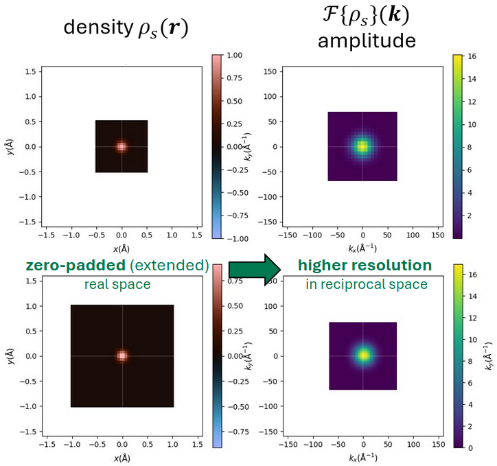
Figure: Larger real space size (achieved for instance by zero padding via the scale_factor attribute) results in a higher resolution in the Fourier reciprocal space.

Phase due to displacement

The dominant feature in the INS spectra, which is the stratification due to the \(\left(1-\cos \left(\mathbf{k} \cdot \mathbf{r}_{a b}\right)\right)\) term, arises in general for any Fourier transform of a repeated displaced object.

Numerically

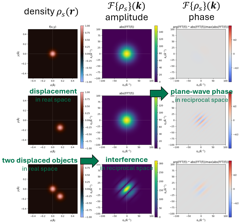
Figure: Displacement results in a plane-wave phase after a Fourier transform. While the FFT amplitude is unchanged if only a single displaced object is present, the interference between the phase of such two objects introduces a plane-wave term in the amplitude.

Analytically

The origin of the \(\left(1-\cos \left(\mathbf{k} \cdot \mathbf{r}_{a b}\right)\right)\) term can be easily shown to come from the Fourier transform of two identical functions with opposite sign displaced in space by vector \(\mathbf{r}_{a b}\) relative to each other

\[\begin{align*} \mathcal{F}\left\{ \; \rho_\mathrm{s} (\mathbf{r}) - \rho_\mathrm{s} (\mathbf{r}-\mathbf{r}_{a b}) \; \right\} = \mathcal{F}\left\{\rho_\mathrm{s} (\mathbf{r})\right\} - \mathcal{F}\left\{\rho_\mathrm{s} (\mathbf{r}-\mathbf{r}_{a b}) \right\} \end{align*}\]

By substitution \(\mathbf{r'} \equiv \mathbf{r}-\mathbf{r}_{a b}\) we have

\[\begin{split}\begin{align*} \mathcal{F}\left\{\rho_\mathrm{s} (\mathbf{r}-\mathbf{r}_{a b}) \right\} &= \int e^{i \mathbf{k} \cdot \mathbf{r}} \rho_\mathrm{s} (\mathbf{r}-\mathbf{r}_{a b}) \mathrm{d}\mathbf{r} = \int e^{i \mathbf{k} \cdot (\mathbf{r'}+\mathbf{r}_{a b})} \rho_\mathrm{s} (\mathbf{r'}) \mathrm{d}\mathbf{r'} \\ &= e^{i \mathbf{k} \cdot \mathbf{r}_{a b}} \; \mathcal{F}\left\{\rho_\mathrm{s} (\mathbf{r}) \right\} \end{align*}\end{split}\]

so that

\[\begin{align*} \mathcal{F}\left\{\rho_\mathrm{s} (\mathbf{r}) - \rho_\mathrm{s} (\mathbf{r}-\mathbf{r}_{a b}) \right\} = \left( 1 - e^{i \mathbf{k} \cdot \mathbf{r}_{a b}} \right) \mathcal{F}\left\{\rho_\mathrm{s} (\mathbf{r}) \right\} \end{align*}\]

and because

\[\begin{align*} \left( 1 - e^{i \mathbf{k} \cdot \mathbf{r}_{a b}} \right) = e^{i \mathbf{k} \cdot \frac{\mathbf{r}_{a b}}{2}} \left( e^{-i \mathbf{k} \cdot \frac{\mathbf{r}_{a b}}{2}} - e^{i \mathbf{k} \cdot \frac{\mathbf{r}_{a b}}{2}}\right) = e^{i \mathbf{k} \cdot \frac{\mathbf{r}_{a b}}{2}} \left(-2i \, \mathrm{sin}(\mathbf{k} \cdot \frac{\mathbf{r}_{a b}}{2})\right) \end{align*}\]

it follows that

\[\begin{split}\begin{align*} \left| \left( 1 + e^{i \mathbf{k} \cdot \mathbf{r}_{a b}} \right) \right|^2 &= \left|e^{i \mathbf{k} \cdot \frac{\mathbf{r}_{a b}}{2}}\right|^2 \cdot \left| -2i \, \mathrm{sin}(\mathbf{k} \cdot \frac{\mathbf{r}_{a b}}{2}) \right|^2 \\ &= 1 \cdot 4 \, \mathrm{sin}^2(\mathbf{k} \cdot \frac{\mathbf{r}_{a b}}{2}) \\ &= 1 \cdot 2 \left(1 - \mathrm{cos}(\mathbf{k} \cdot \mathbf{r}_{a b})\right) \end{align*}\end{split}\]

using the identity \(\mathrm{sin}^2(x) = \frac{1}{2} (1 - \mathrm{cos}(2x))\); hence

\[\begin{align*} \left|\mathcal{F}\left\{\rho_\mathrm{s} (\mathbf{r}) - \rho_\mathrm{s} (\mathbf{r}-\mathbf{r}_{a b}) \right\}\right|^2 = 2 \, \left(1 - \mathrm{cos}(\mathbf{k} \cdot \mathbf{r}_{a b})\right) \; |\mathcal{F}\left\{\rho_\mathrm{s} (\mathbf{r}) \right\}|^2 \,. \end{align*}\]

Further details

Please see L. Spitz, L. Vojáček, et al., under preparation for further details on the theory and the implementation of the present package.