Examples#
Example of use is given in ./examples/example_of_use.ipynb in the examples folder.
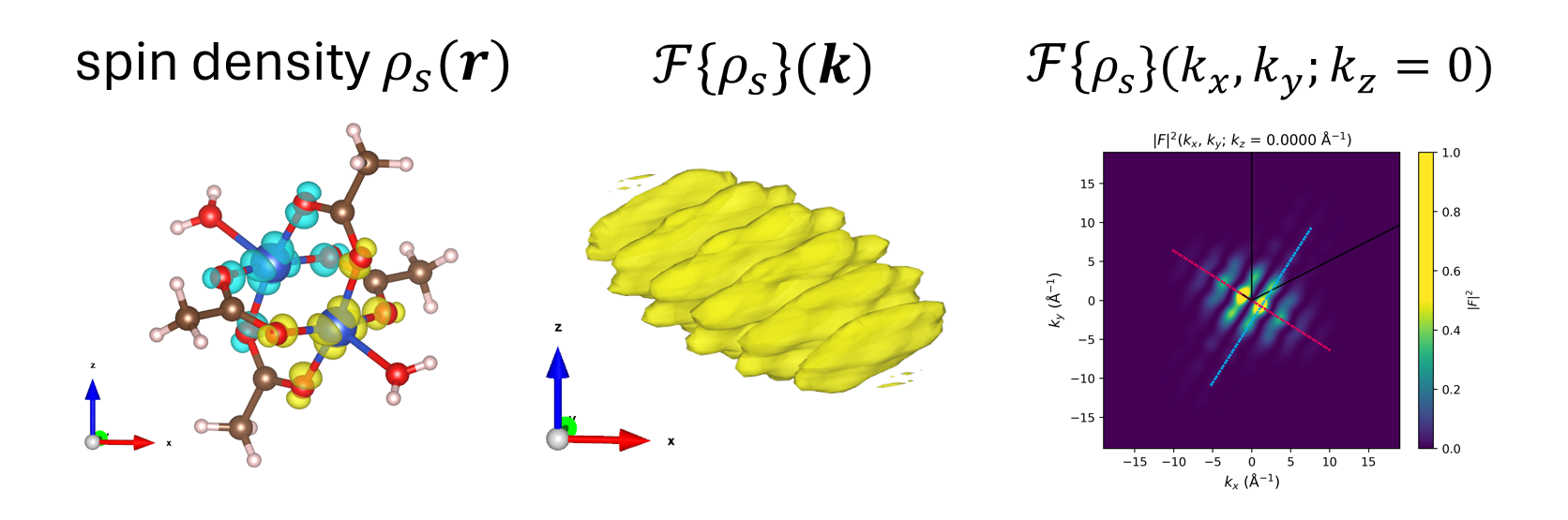
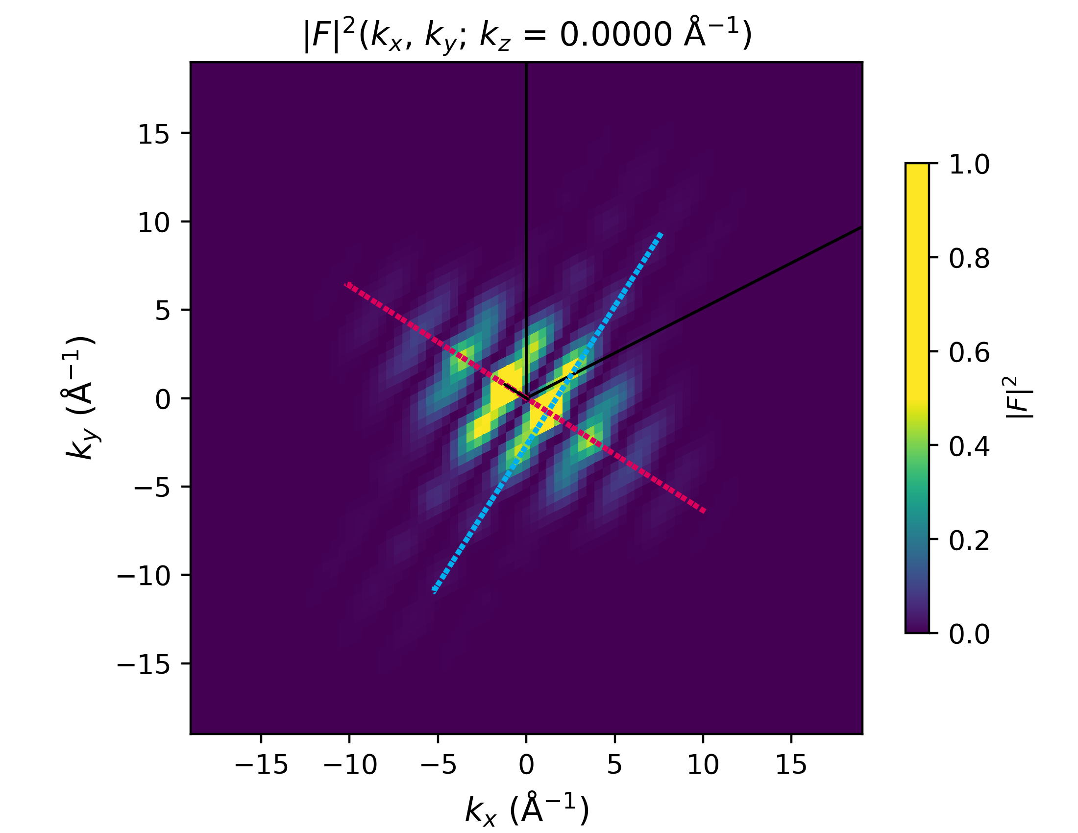
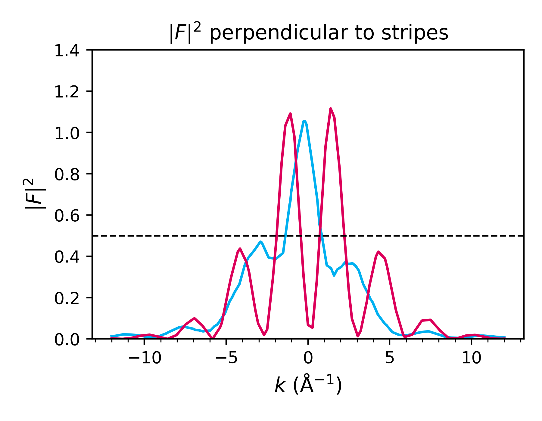
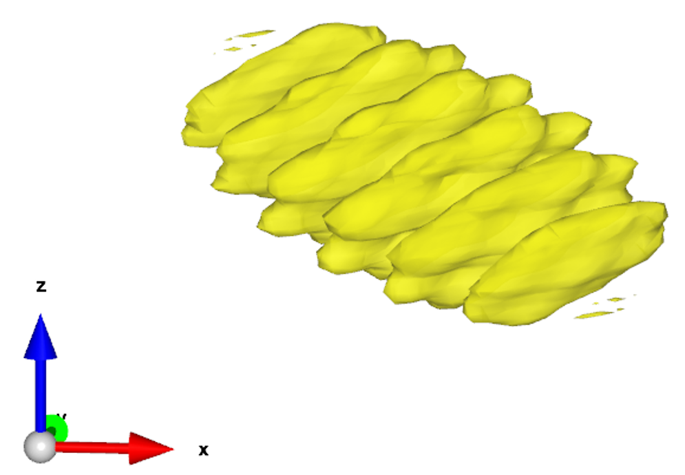
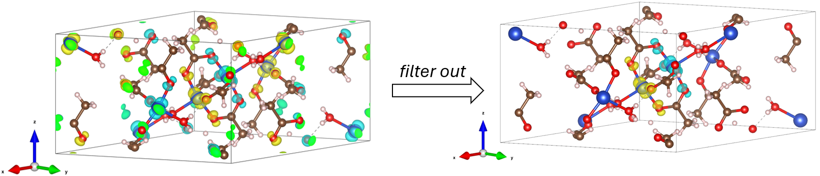
Figure: Example of use of the fft_electronic_spin_density package. Left: The input is a Gaussian .cube file of charge density. Middle: The output is a .cube file of its Fourier transform (—> visualize in VESTA). Right: The Fourier transform is visualized in 3D, 2D, and 1D cuts. The original DFT density can be manipulated by filtering it out only around selected sites, replacing by a model and even fitting this model to the original density.#
Import the Density class#
from fft_electronic_spin_density.classes import Density
Load the (spin) density .cube file#
density = Density(fname_cube_file='../cube_files/Cu2AC4_rho_sz_256.cube')
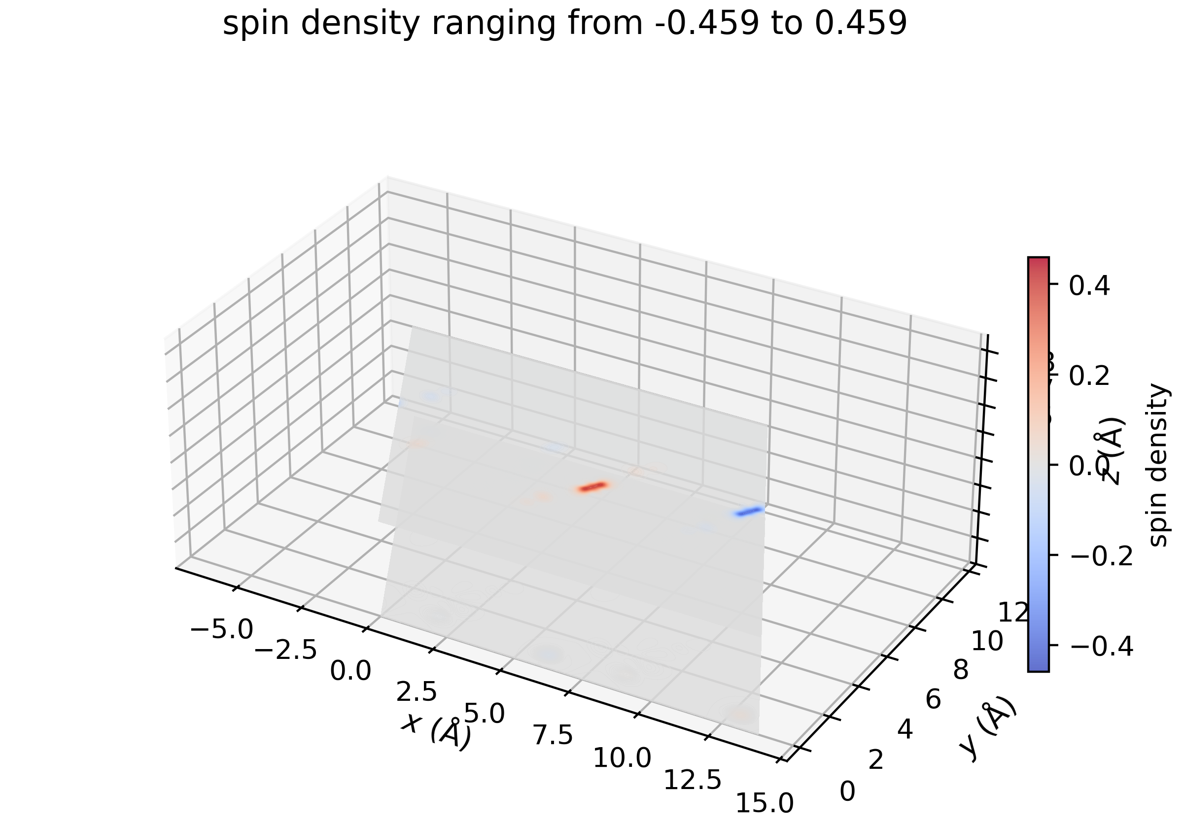
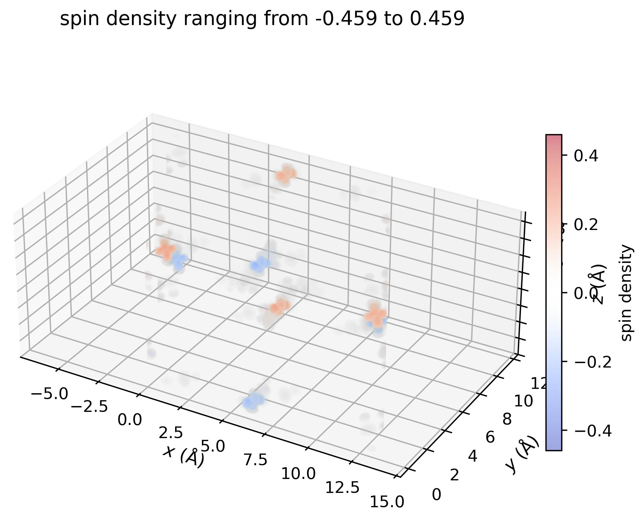
Visualize the density in 3D#
density.plot_cube_rho_sz(
                    c_idx_arr=np.arange(0, density.nc),
                    fout_name='rho_sz_exploded.jpg',
                    alpha=0.05,
                    figsize=(5.5,5.5),
                    dpi=400,
                    zeros_transparent=True,
                    show_plot=True
                    )
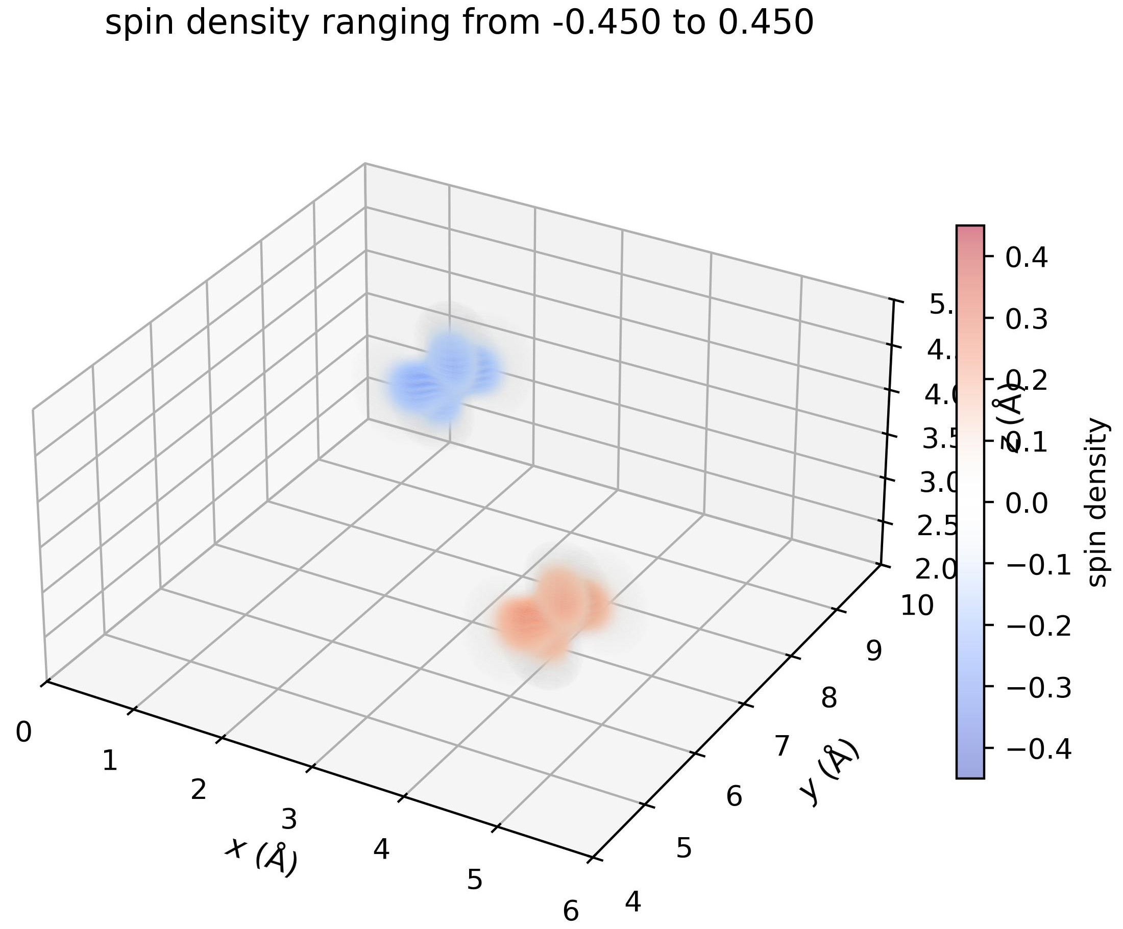
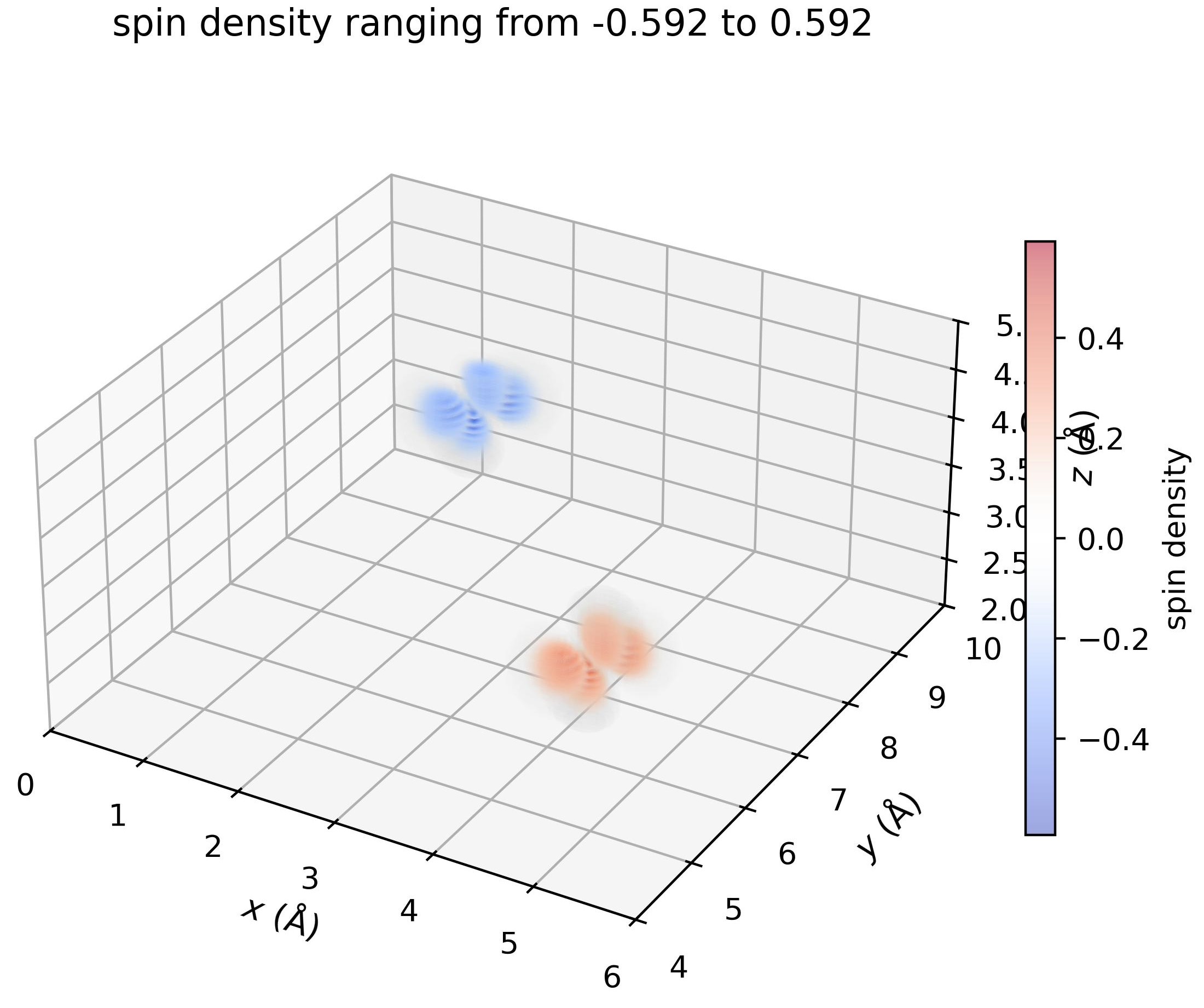
Filter out \(\rho_\mathrm{s} (\mathbf{r})\) around selected sites#
# selected site indices
site_idx = [0, 1] # atom 0 - Cu0, atom 1 - Cu1

# muffin-tin radii around the selected sites where density will be kept
site_radii = [1.1]*2 # Angstrom

density.mask_except_sites(leave_sites={
                            'site_centers':density.get_sites_of_atoms(site_idx),
                            'site_radii':site_radii
                            })
and visualize…
density.plot_cube_rho_sz(
                 c_idx_arr=np.arange(0, density.nc, 1),
                 fout_name='rho_sz_exploded_filtered.jpg',
                 alpha=0.05,
                 figsize=(5.5,5.5),
                 dpi=400,
                 zeros_transparent=True,
                 show_plot=True,
                 xlims=[0, 6],
                 ylims=[4,10],
                 zlims=[2,5]
                 )
Perform FFT, visualize in 2D and 1D#
density.FFT()
and visualize:
fft_along_line_data = density.plot_fft_along_line(
                                i_kz=density.nkc//2,
                                cut_along='both',
                                kx_ky_fun=None,
                                k_dist_lim=12,
                                N_points=3001,
                                fout_name='cut_1D_both.png',
                                cax_saturation=0.5,
                                )

kx_arr_along, ky_arr_along, F_abs_sq_interp_along, \
kx_arr_perp, ky_arr_perp, F_abs_sq_interp_perp = fft_along_line_data

density.plot_fft_2D(
            i_kz=density.nkc//2,
            fft_as_log=False,
            fout_name=f'F_abs_sq-scale_kz_at_idx_{density.nkc//2}_cut_both.png',
            figsize=(5.5, 4.5),
            dpi=400,
            fixed_z_scale=True,
            cax_saturation=0.5,
            xlims=[-19, 19],
            ylims=[-19, 19],
            zlims=[0, 1.6e6],
            plot_line_cut=True, kx_arr_along=kx_arr_along, ky_arr_along=ky_arr_along,
            kx_arr_perp=kx_arr_perp, ky_arr_perp=ky_arr_perp,
            cut_along='both'
            )
Write out \(\mathcal{F}\{ \rho_\mathrm{s} \}\) as a .cube file#
density.write_cube_file_fft(fout='fft_rho_sz.cube')
→ visualize the .cube file in VESTA
Replace \(\rho_\mathrm{s} (\mathbf{r})\) by a model#
The model is defined as a dx2y2 orbital centered on Cu sites. Possibly, sp orbitals centered on oxygen sites can be added. Any parameterized function (e.g., a Gaussian) can be defined as a model.
site_idx = [0, 1]

parameters_model = {'type':['dx2y2_neat']*2,
                    'sigmas':[None]*2,
                    'centers':density.get_sites_of_atoms(site_idx),
                    'spin_down_orbital_all':[False, True],
                    'fit_params_init_all':{
                        'amplitude':[0.3604531, 0.3604531],
                        'theta0':   [-1.011437, -1.011437],
                        'phi0':     [-0.598554, -0.598554],
                        'Z_eff':    [12.848173, 12.848173],
                        'C':        [0.0000000, 0.0000000]
                        }
                    }

density.replace_by_model(
                    fit=False,
                    parameters=parameters_model
                    )
density.plot_cube_rho_sz(
                    c_idx_arr=np.arange(0, density.nc, 1),
                    fout_name='rho_sz_exploded_model.jpg',
                    alpha=0.05,
                    figsize=(5.5,5.5),
                    dpi=400,
                    zeros_transparent=True,
                    show_plot=True,
                    xlims=[0, 6],
                    ylims=[4,10],
                    zlims=[2,5]
                    )
Fit a model to the original density#
site_idx = [0, 1]

parameters_model = {'type':['dx2y2_neat']*2,
                    'sigmas':[None]*2,
                    'centers':density.get_sites_of_atoms(site_idx),
                    'spin_down_orbital_all':[False, True],
                    'fit_params_init_all':{
                        'amplitude':[0.3604531, 0.3604531],
                        'theta0':   [-1.011437, -1.011437],
                        'phi0':     [-0.598554, -0.598554],
                        'Z_eff':    [12.848173, 12.848173],
                        'C':        [0.0000000, 0.0000000]
                        }
                    }

density.replace_by_model(
                    fit=True,
                    parameters=parameters_model
                    )
Write out the modified \(\rho_\mathrm{s} (\mathbf{r})\)#
At any stage of filtering out, replacing by a model or fitting:
density.write_cube_file_rho_sz(fout='rho_sz_modified.cube')
… to be visualized in VESTA
Integrate \(\rho_\mathrm{s} (\mathbf{r})\) over the unit cell#
rho_tot_unitcell, rho_abs_tot_unitcell = density.integrate_cube_file(verbose=False)

print(f"""Total charge in the unit cell {rho_tot_unitcell:.4f} e.
Total absolute charge in the unit cell {rho_abs_tot_unitcell:.4f} e.""")
Visualize the density as 2D slices#
at selected heights (z-coordinates) along the $c$ lattice vector:
# z position of atom 0
site_coordinates = density.get_sites_of_atoms(site_idx=[0])
atom_0_z_coordinate = site_coordinates[0][2]

# indices along the c lattice vector where density cuts should be plotted
c_idx = density.get_c_idx_at_z_coordinates(z_coordinates=[0.0, atom_0_z_coordinate])

density.plot_cube_rho_sz(
                    c_idx_arr=c_idx,
                    fout_name='rho_sz_exploded_masked.jpg',
                    alpha=0.8,
                    figsize=(6.0, 4.5),
                    dpi=400,
                    zeros_transparent=False,
                    show_plot=True
                    )