Example#

An example of use is given in ./examples/one-dimensional_channel.ipynb.

There is also a time-complexity study in ./examples/time_complexity.ipynb.

1. Linear-chain tight-binding Hamiltonian#

from fuNEGF.models import LinearChain
import numpy as np

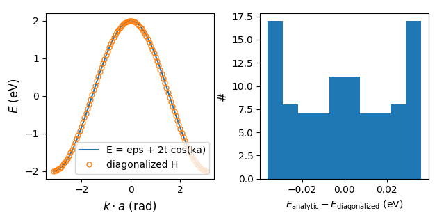
chain = LinearChain(N=100, eps_0=0.0, t=1.0, a=1.0, H_impurity=None, plot_dispersion=True)

_images/linear_chain_dispersion_analytic_vs_diagonalized.png

2. Impurity potential#

H_impurity = np.zeros((N, N), dtype=complex)

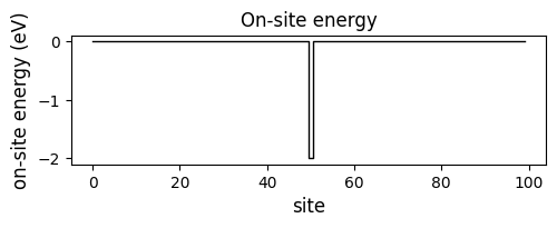
# (1) add a single impurity in the middle
H_impurity[N // 2, N // 2] += -2 * t

chain.add_H_impurity(H_impurity, plot_dispersion=False)
chain.plot_onsite_energy()

3. Chemical potential with impurities#

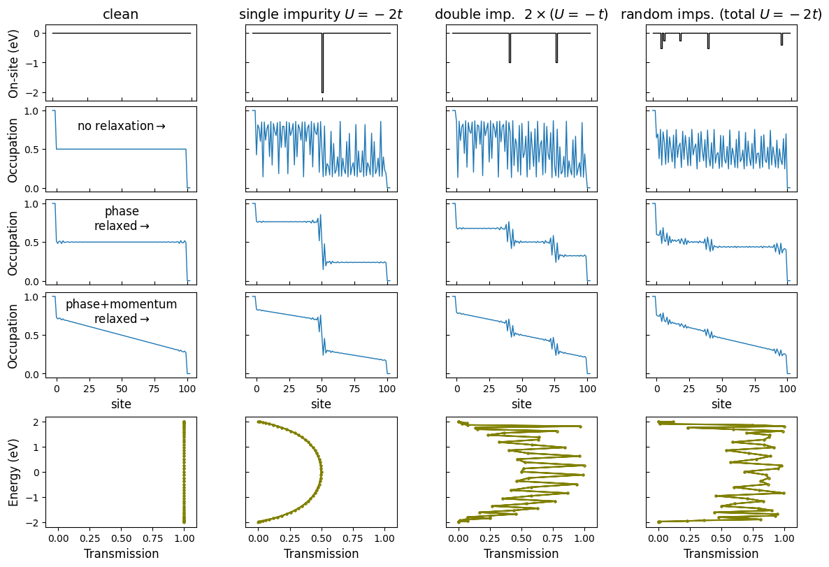
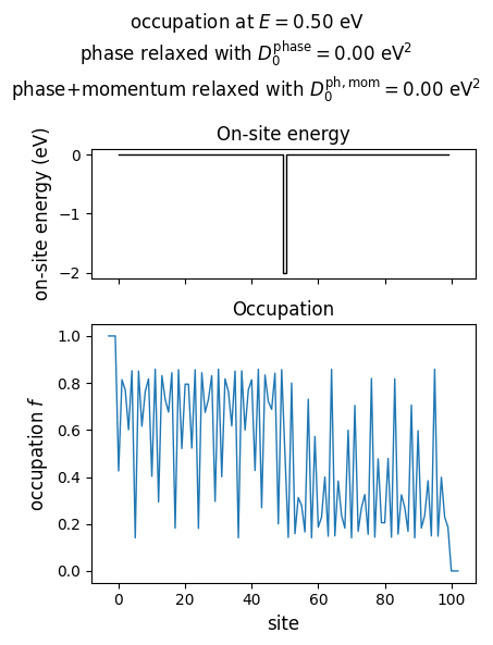
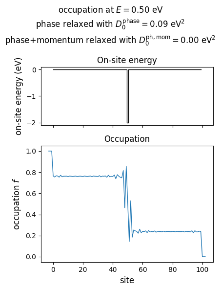
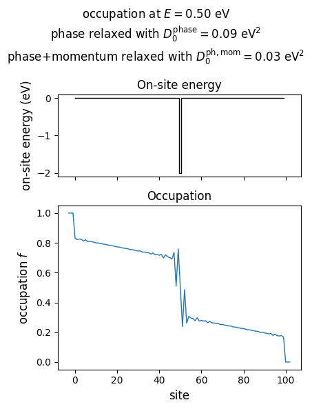
There is a potential drop at the impurities - the impurities act as quantum resistors in series. This can be demonstrated by calculating the occupation function profile.

3.1. No relaxation#

Without any relaxation mechanism, strong resonances arise, making the potential drop unclear.

# no relaxation
D0_phase = 0.00 * t**2
D0_phase_momentum = 0.00 * t**2

plot_onsite_and_occupation(E_to_plot, D0_phase, D0_phase_momentum, N_sc)

_images/single_imp_middle_no_relaxation.png

3.2. Phase relaxation#

Phase relaxation attenuates the Fabry-Pérot resonances.

# only phase
D0_phase = 0.09 * t**2
D0_phase_momentum = 0.00 * t**2

plot_onsite_and_occupation(E_to_plot, D0_phase, D0_phase_momentum, N_sc)

_images/single_imp_middle_phase_relaxation.png

3.3. Phase and momentum relaxation#

With an additional momentum relaxation, the potential drop is partially distributed over the whole channel length.

# phase and momentum
D0_phase = 0.09 * t**2
D0_phase_momentum = 0.03 * t**2

plot_onsite_and_occupation(E_to_plot, D0_phase, D0_phase_momentum, N_sc)

_images/single_imp_middle_phase_and_momentum_relaxation.png

4. Transmission function#

The transmission function reads

\[\bar{T}(E)=\operatorname{Trace}\left[\boldsymbol{\Gamma}_1 \mathbf{G}^R \boldsymbol{\Gamma}_2 \mathbf{G}^A\right].\]

4.1. Single impurity#

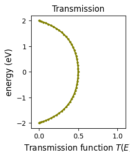
A single impurity in the center

H_impurity = np.zeros((N, N), dtype=complex)
H_impurity[N // 2, N // 2] += -2 * t
chain.add_H_impurity(H_impurity, plot_dispersion=False)

chain.plot_transmission()

reduces the transmission from the clean limit \(T(E) = 1.0\) to (at most) half of that value \(T(E=0.0) = 0.5\):

_images/transmission_single_imp_middle.png

4.2. Different impurity distributions#

Let us now compare the transmission for several cases.

Without impurities, the transmission function is constant \(T(E) = 1.0 = \mathrm{const.}\).
With a single impurity of \(U=-2.0 t\), the transmission reaches at most the half of the clean-limit maximum \(T(E=0.0) = 0.5\).
With two impurities of \(U=-t\) each, the function looks almost the same but with strong resonances.
With many distributed impurities of equivalent total strength \(\Sigma_i U_i = -2.0 t\), the transmission starts to resemble the clean limit \(T(E) = 1.0 = \mathrm{const.}\)

# RELAXATION
D0_phase = 0.12 * t**2
D0_phase_momentum = 0.03 * t**2
N_sc = 90

# IMPURITY HAMILTONIANS
H_imp_clean = np.zeros((N, N))
H_imp_single = np.zeros((N, N))
H_imp_single[N // 2, N // 2] = -2 * t
...

H_impurities = [H_imp_clean, H_imp_single, H_imp_double, H_imp_multiple]

# CALCULATE AND PLOT
fig, axes = plt.subplots(5,len(H_impurities))

for i, H_imp in enumerate(H_impurities):
   chain = LinearChain(N, eps_0, t, a, H_impurity=H_imp, plot_dispersion=False)
   chain.plot_onsite_energy(axes[0, i])
   chain.plot_occupation(
      D0_phase=0, D0_phase_momentum=0, E_to_plot=E_to_plot, N_sc=N_sc, ax=axes[1, i]
   )
...

Example

Contents